

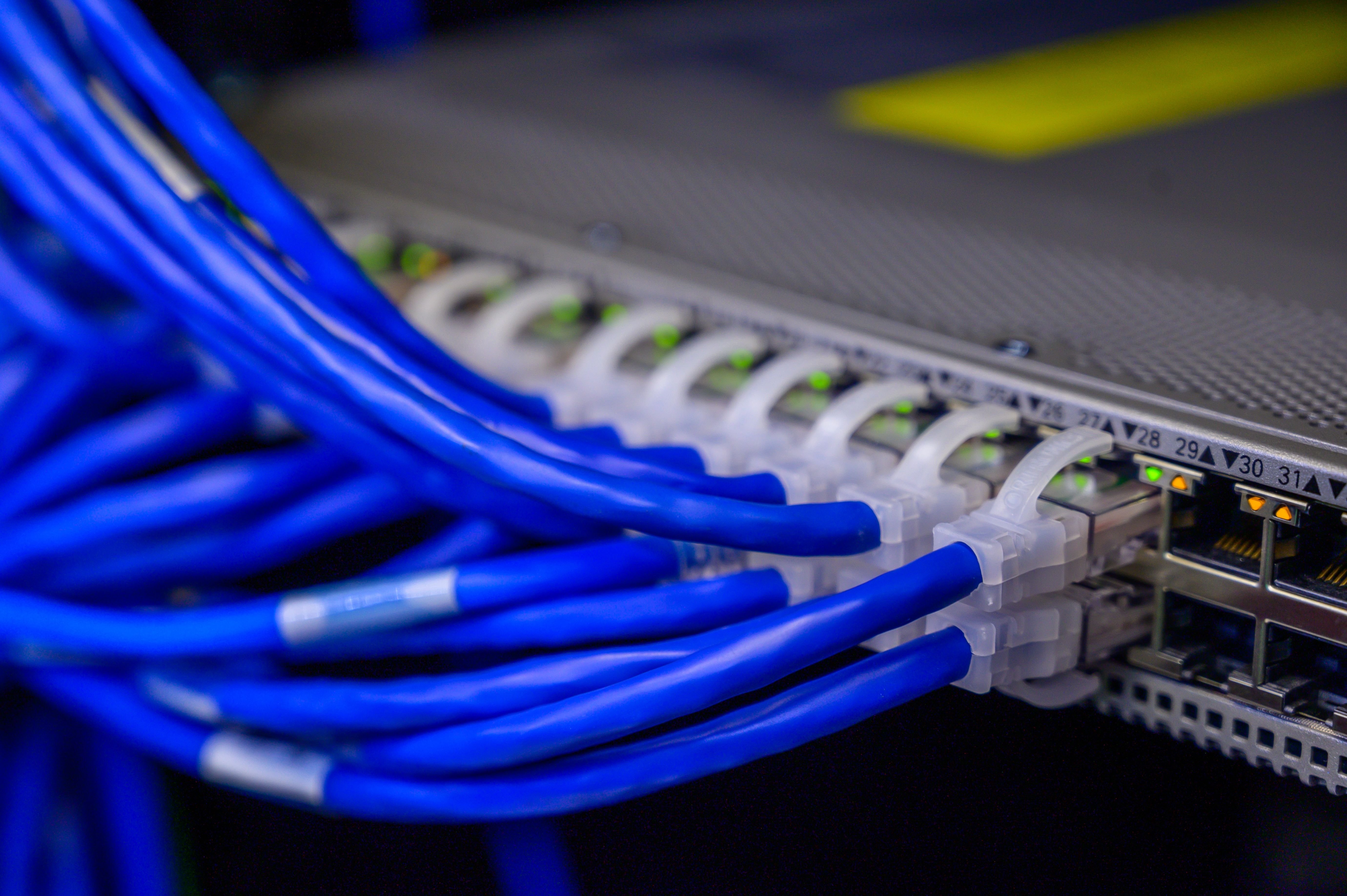
Adding a second network interface feels like an obvious reliability improvement. If one interface fails, traffic moves to the other. Bond two links together and perhaps you gain both redundancy and additional throughput. Put several paths between systems and losing one path should no longer matter.
That reasoning is directionally correct, but it is incomplete. A redundant link protects against a specific failure: the loss of that link or path. It does not automatically protect against an overloaded CPU, a shared upstream switch, a congested queue, a packet-inspection engine that cannot keep up, an interrupt path pinned to one saturated core, a flow hash that concentrates traffic on one interface, or a downstream service whose capacity is lower than the network feeding it.
This distinction became much clearer to me while building a Raspberry Pi 5 networking testbed for repeatable throughput, resilience, and packet-inspection experiments. I benchmarked physical interfaces and Linux NIC bonding, generated controlled traffic with iperf3 and hping3, measured Suricata inspection behavior, and correlated network results with CPU utilization, memory, interrupts, interface counters, packet drops, and end-to-end throughput.
The interesting question quickly stopped being:
“Do I have two links?”
and became:
“What resource actually limits the system after one of those links fails?”
That is a much more useful way to think about redundancy, because sometimes the redundant component behaves exactly as designed and the system still falls over.
Redundancy and Capacity Are Different Properties
Suppose a machine has two 1 Gbps Ethernet interfaces. It is tempting to describe the system as:
1 Gbps + 1 Gbps = 2 Gbps
but that result depends entirely on how the interfaces are configured and how traffic can actually be distributed across them.
Linux bonding supports several operating modes. Some are primarily about failover, while others attempt to distribute traffic. Active-backup bonding is a good example of why those goals need to be separated:
Both interfaces exist, but only one normally carries traffic. If eth0 fails, eth1 takes over.
The capacity model is therefore roughly:
Normal capacity:  1 Gbps
Failure capacity: 1 Gbps
not:
Normal capacity: 2 Gbps
The point of active-backup is resilience, not bandwidth aggregation.
Other bonding modes can distribute traffic, but even there aggregate link capacity does not imply that every connection can use every link at once. Flow affinity, hashing policy, switch behavior, and the number of independent flows all matter.
That leads to the first important distinction:
Redundancy asks whether traffic has somewhere else to go. Capacity asks whether that alternative can handle the traffic that moves there.
Those are separate properties, and a system can satisfy one while failing the other.
Failover Can Work and Still Cause an Outage
Imagine a service carrying 1.6 Gbps across two 1 Gbps paths:
In the healthy state, nothing looks wrong. Both links operate below capacity.
Then Link A disappears:
The redundancy mechanism may behave perfectly. Routes change or traffic moves to Link B exactly as the system was designed to do.
The problem is that 1.6 Gbps of offered load is now trying to cross a path capable of roughly 1 Gbps.
The first visible symptom may be queue growth. Latency then increases. Buffers eventually fill, packets drop, TCP retransmits, and application throughput deteriorates.
From the component's perspective:
Failover: SUCCESS
From the user's perspective:
System: DEGRADED OR DOWN
That is why redundancy needs to be tested under failure load, not merely by unplugging a cable and confirming that a ping still succeeds.
The meaningful question is:
Does the surviving end-to-end path have enough capacity
to absorb the required workload after the failure?
A backup path that can carry control traffic but not production traffic is technically redundant and operationally insufficient.
Alternate Paths Still Need Capacity
A useful larger-scale example came from a Cloudflare incident involving heavy traffic associated with AWS us-east-1.
According to Cloudflare's incident account, direct peering capacity became saturated. Routing changes moved traffic toward additional paths, but those alternate paths also encountered capacity limits. Cloudflare described existing reduced capacity on part of the direct peering infrastructure and an interconnect involved in the alternate route that was awaiting additional capacity. As queues grew, packet loss followed.
Conceptually, the failure looked like this:
The important lesson is not merely that congestion occurred. The topology had alternate paths. Routing moved traffic. The redundancy mechanism had somewhere else to send work.
The alternate infrastructure still did not have enough failure-state capacity for the traffic it inherited.
An alternate path only provides useful redundancy if its failure-mode capacity is sufficient for the workload that may move onto it.
That principle applies to hyperscale peering links, but it also applies to two Ethernet adapters connected to a small Linux machine.
The Bottleneck May Not Be the Link
Suppose I successfully increase the amount of traffic entering a machine by bonding interfaces.
That does not mean the machine can process twice as much useful traffic.
The actual path looks more like this:
Every stage has finite capacity.
If the interfaces can collectively receive 2 Gbps but Suricata can inspect only 900 Mbps for a particular packet distribution and rule set, adding another interface does not create a 2 Gbps inspection system. It creates a faster path into a 900 Mbps processing boundary.
That is why throughput is an end-to-end property rather than a number that belongs to the NIC.
Consider this hypothetical pipeline:
NIC line rate          1.0 Gbps
Kernel processing      1.0 Gbps
Inspection capacity    650 Mbps
Application capacity   800 Mbps
Useful throughput is constrained approximately by:
min(
    NIC,
    kernel,
    inspection,
    application
)
which gives:
650 Mbps
Now add another 1 Gbps NIC. Network ingress capacity may become:
NIC capacity = 2 Gbps
while inspection remains:
Inspection capacity = 650 Mbps
Nothing is wrong with the second interface. It simply exposed a bottleneck somewhere else in the pipeline.
Redundancy and additional network capacity can therefore make a system's next constraint more visible without improving the final throughput at all.
Packet Rate Changes the Experiment
Bandwidth by itself is also an incomplete workload description.
These two workloads both move 1 Gbps:
1 Gbps of large packets
and:
1 Gbps of very small packets
but they can impose dramatically different packet-processing costs.
A packet-processing system does not only process bytes. It handles packet descriptors, headers, queues, flow state, protocol tracking, interrupts, memory accesses, rules, and other per-packet work.
At a simplified level:
packets per second ≈ bandwidth / packet size
Smaller packets therefore mean many more packets per second for the same bit rate.
That matters for firewalls, routers, IDS/IPS software, and the kernel itself. A system capable of moving a high bit rate of large packets may hit a packets-per-second ceiling much earlier with smaller frames.
A useful benchmark should therefore vary at least two dimensions:
offered bandwidth
+
packet size
and often several more:
flow count
connection type
traffic direction
protocol mix
In my own testbed, this is why I generated controlled workloads across multiple traffic rates and packet sizes rather than treating one saturated iperf3 run as the complete performance picture.
A benchmark is only meaningful in the context of the workload it represents.
Suricata Adds Another Processing Boundary
Packet inspection makes the pipeline more interesting because incoming traffic now has to be distributed among workers while preserving the semantics of each flow.
Suricata supports multiple worker threads, with packet-capture mechanisms helping distribute traffic across them. Its documentation emphasizes that packet distribution matters not only for performance but also for correctness: packets belonging to a flow need to be handled consistently enough that stateful inspection works as intended.
A simplified model looks like this:
On paper, this looks ideal: four receive queues, four workers, four CPU cores.
But that architecture only helps if the workload can actually distribute across those queues and workers.
Traffic is rarely perfectly balanced. A single dominant flow, uneven hashing, interrupt affinity, queue configuration, or worker placement can leave one execution path saturated while another core remains lightly used.
Parallelism gives the system more places to perform work.
It does not guarantee that the workload can use them evenly.
RSS Helps, but Hashing Does Not Guarantee Balance
Modern NICs often support Receive Side Scaling, or RSS. The NIC hashes selected packet metadata and uses the result to place flows onto receive queues, which can then be handled by different CPUs.
Conceptually:
The key word is flows.
Suppose the traffic consists of:
Flow A: 700 Mbps
Flow B: 100 Mbps
Flow C: 100 Mbps
Flow D: 100 Mbps
Even with four queues, the 700 Mbps flow may remain assigned to one queue because preserving flow ordering is important.
The resulting utilization could look like:
CPU 1: ████████████████████ 100%
CPU 2: ███                  20%
CPU 3: ██                   15%
CPU 4: ███                  20%
The machine still has unused aggregate CPU capacity.
The overloaded flow does not.
This is an important performance distinction. A system can appear underutilized at the machine level while one packet-processing path has already reached its ceiling.
That is another way redundancy or parallelism can appear available on paper while offering little benefit to the particular workload causing the problem.
More Workers Do Not Automatically Mean More Throughput
A common response to CPU pressure is:
CPU overloaded?
Add threads.
Sometimes that works.
Sometimes it exposes another bottleneck.
Suricata's performance guidance ties together NIC queues, RSS, interrupt handling, CPU affinity, worker placement, NUMA locality, driver behavior, and hardware topology because the pipeline behaves as a system rather than as a collection of independent thread counts.
The path is closer to:
NIC queues
    ↓
interrupt distribution
    ↓
CPU locality
    ↓
worker scheduling
    ↓
cache behavior
    ↓
inspection cost
Adding workers beyond what the queue topology or workload can effectively feed may produce diminishing returns. Eventually the system can start paying more for scheduling, cache misses, lock contention, memory bandwidth, cross-core communication, or NUMA effects than it gains from additional parallelism.
That leads to a useful performance principle:
Parallelism exposes available resources. It does not manufacture capacity that the rest of the pipeline cannot use.
The right worker count is therefore not necessarily "as many as possible." It is the number that works with the actual queue, CPU, memory, and traffic topology of the system.
Watch Interrupts, Queues, and Drops
Network benchmarking becomes far more useful once the experiment includes system-level instrumentation.
A minimal test might record only:
iperf3 throughput
A more useful one also watches:
CPU utilization
per-core utilization
memory utilization
packet drops
interrupt counts
interface counters
Suricata statistics
latency
queue behavior
For example, I might generate controlled traffic with:
iperf3 -c 192.168.1.20 -P 4 -t 60
while also inspecting:
cat /proc/interrupts
and:
ip -s link show eth0
and, when the driver exposes useful counters:
ethtool -S eth0
The purpose is not to collect metrics because more charts look impressive.
It is to answer:
Where did the work actually go?
Suppose aggregate utilization reports:
CPU usage: 42%
That sounds comfortable.
The per-core view may instead be:
CPU0: 100%
CPU1: 24%
CPU2: 20%
CPU3: 24%
Now the result means something very different. One packet-processing or interrupt path may be saturated even though most of the machine remains idle.
Aggregate metrics are useful summaries.
They are dangerous when the bottleneck is localized.
Buffers Can Hide Overload
Queues often provide the first visible indication that one stage of the pipeline cannot keep up.
When:
arrival rate > processing rate
the extra work has to wait somewhere.
The progression is typically:
queue grows
    ↓
latency grows
    ↓
queue fills
    ↓
packets drop
The same pattern can happen in a router, kernel receive path, application queue, or packet-inspection system.
Increasing the queue size may delay packet loss. It does not necessarily increase steady-state processing capacity.
That distinction matters because larger buffers can make a benchmark appear healthier while users experience worse latency.
Imagine a processor that can sustainably handle:
800 Mbps
while traffic arrives at:
1 Gbps
A larger buffer can initially produce:
fewer immediate drops
but those packets are accumulating somewhere. Eventually the tradeoff becomes:
larger queue
→ absorbs burst
→ fewer immediate drops
→ potentially higher queueing latency
versus:
smaller queue
→ earlier drops
→ less buffered work
→ faster overload signal
Neither is universally correct.
A system designed for short bursts may benefit from buffering. A latency-sensitive application may prefer a different tradeoff. Sustained overload requires increasing processing capacity or reducing load rather than merely increasing how much excess traffic can wait.
Buffers handle bursts.
They do not repeal queueing theory.
Failure Detection Is Part of Redundancy
Even active-backup bonding hides another question:
How does the system know that the active path failed?
Linux bonding can use link-monitoring mechanisms such as MII monitoring or ARP-based monitoring. Without appropriate health detection, the driver may continue believing that an interface is usable even when the path beyond it is not.
That matters because these states are not equivalent:
NIC electrically up
Switch port up
End-to-end path healthy
Consider:
NIC is UP
Switch port is UP
Upstream forwarding path is broken
A carrier-level check can still report:
link = UP
while useful traffic has nowhere to go.
Redundant interfaces therefore do not automatically imply fast or correct failure detection.
The broader distributed-systems principle is familiar:
You cannot fail over from a failure you cannot detect.
The health signal has to represent the failure domain you care about. Detecting that a cable is connected is enough for cable failure. It is not enough to prove that the application can still reach its dependency.
Two Paths Can Still Share One Failure Domain
Another common weakness is shared fate.
Suppose a host has two NICs:
There is interface redundancy.
There is no switch redundancy.
If that switch fails, both paths disappear together.
The same pattern continues higher in the topology:
two switches
→ same router
or:
two routers
→ same power circuit
or:
two routes
→ same constrained interconnect
may still share one meaningful failure domain.
That is why counting interfaces or drawing two arrows on a topology diagram is not enough. Real redundancy depends on whether the supposedly independent paths fail independently.
The Cloudflare example illustrates this at a much larger scale. Alternate routing existed, but the shifted traffic still encountered shared or insufficient capacity elsewhere in the path.
Redundancy is therefore as much about failure-domain independence as it is about path count.
Bonding Has a Traffic-Distribution Problem
Even when a bonding mode distributes traffic, another question remains:
Distribute according to what?
Depending on the mode and transmit hash policy, traffic distribution can use information such as:
source MAC
destination MAC
source IP
destination IP
source port
destination port
That matters because aggregate capacity is often available across many flows rather than inside one flow.
Imagine thousands of connections between different endpoints. Hashing may spread them reasonably well across two interfaces.
Now imagine one enormous TCP connection between one source and one destination. Depending on the bonding mode and policy, that connection may remain pinned to one physical link so packets are not arbitrarily reordered.
Therefore:
2 × 1 Gbps bonded links
may offer close to 2 Gbps of useful aggregate capacity across a suitable multi-flow workload while one connection remains bounded near:
1 Gbps
That is not necessarily a failure in the bonding implementation.
It is a consequence of the traffic-distribution policy and the need to preserve sensible flow behavior.
The useful question is not:
How many interfaces are present?
It is:
What traffic distribution can this architecture
actually exploit?
The answer depends on the workload.
Benchmark the Failure State
This became the most important practical lesson from my redundancy experiments.
A healthy-state benchmark such as:
two links active
→ measure throughput
is useful.
It is not enough.
The more revealing experiment is:
two links active
→ establish sustained load
→ fail one link
→ measure what changes
And the result should include much more than throughput.
I want to observe:
packet loss
latency
recovery time
interrupt distribution
CPU utilization
queue behavior
inspection drops
application errors
A broader experiment matrix can expose different bottlenecks:
| Scenario | What it reveals |
|---|---|
| Single interface, no inspection | Baseline network capacity |
| Bonded interfaces, no inspection | Bonding behavior |
| Bonded interfaces, one link removed | Failover characteristics |
| Single interface + Suricata | Inspection cost |
| Bonded interfaces + Suricata | Whether inspection becomes the bottleneck |
| Small packets | Packet-processing ceiling |
| Large packets | Bandwidth ceiling |
| One large flow | Hash and flow-affinity behavior |
| Many parallel flows | Load-distribution behavior |
| CPU/IRQ pinning changes | Processing locality |
| Sustained overload | Queue growth and drop behavior |
Now the benchmark begins answering architectural questions instead of merely producing a larger number.
The most useful failure experiment is not "does traffic continue?"
It is:
What resource becomes limiting after traffic continues?
That is the point where redundancy testing becomes resilience testing.
Reproducibility Matters More Than One Impressive Number
Networking benchmarks are highly sensitive to configuration.
Change any of these:
packet size
flow count
CPU affinity
kernel version
NIC driver
firmware
inspection rules
queue size
bond mode
offloading
and the result may change.
Suricata's own performance guidance warns that changes to drivers, firmware, kernel behavior, and system configuration can influence packet-processing results. That is why a reproducible harness is more useful than a screenshot showing:
941 Mbps
with no context.
A useful test record includes:
hardware
software versions
kernel version
bond mode
traffic-generation command
test duration
packet size
flow count
inspection rules
CPU affinity
queue configuration
results
Then a future experiment can answer:
Did this configuration change improve the same workload?
instead of:
Why is today's benchmark different from the number I remember seeing last week?
Performance engineering becomes much more valuable when tests can be repeated under controlled conditions.
An impressive number is evidence once.
A reproducible experiment can become evidence again.
Capacity Planning Needs the Failure Topology
Normal-state capacity planning asks:
Can the system handle today's traffic?
Resilience planning asks:
Can the system handle today's traffic
after losing something?
Those are different questions.
Suppose production normally operates at:
70% of total aggregate capacity
across two equal paths.
If one path disappears and total available link capacity is cut in half, the surviving path may suddenly be asked to carry the equivalent of:
140% of its capacity
The architecture is redundant.
The capacity plan is not.
A more useful model asks about N-1 capacity:
What happens when one expected component is unavailable?
Depending on the system, the component might be:
one interface
one link
one switch
one router
one peering interconnect
one processing node
one availability zone
The unit changes.
The reasoning does not.
Failure-state capacity needs to be intentional. Otherwise redundancy may simply ensure that traffic survives long enough to overwhelm the next component.
Find the Point Where Throughput Stops Scaling
One of the most revealing experiments is to increase offered load gradually.
For example:
100 Mbps
300 Mbps
500 Mbps
700 Mbps
900 Mbps
1.1 Gbps
Early in the test, processed throughput may scale linearly:
offered:   500 Mbps
processed: 500 Mbps
Later:
offered:   900 Mbps
processed: 820 Mbps
and eventually:
offered:   1.1 Gbps
processed: 825 Mbps
That plateau matters.
The system is telling you that something downstream has reached capacity.
The next step is to correlate the plateau with lower-level measurements:
CPU utilization
per-core utilization
interrupts
queue drops
Suricata stats
NIC counters
latency
Perhaps the result is:
NIC drops:         0
CPU core 2:      100%
Suricata drops: increasing
Now the diagnosis is much more useful than:
network is slow
The links may be completely healthy. The NIC may have no drops. One CPU and the inspection engine may be the actual ceiling.
The purpose of instrumentation is therefore not simply observability.
It is bottleneck localization.
When Redundancy Fails at the System Level
Redundancy does not necessarily fail because the backup component itself breaks.
It can fail its system-level purpose in several different ways.
The backup lacks failure-state capacity
Traffic moves exactly as designed, but the surviving path cannot absorb the inherited load.
Multiple paths share the same failure domain
Two NICs feed one switch, two switches feed one router, or several routes eventually converge on the same constrained interconnect.
The bottleneck is downstream
The network can deliver packets faster than CPU, inspection, storage, or the application can consume them.
Traffic cannot distribute evenly
Flow hashing concentrates a dominant workload on one NIC, receive queue, interrupt path, worker, or CPU.
Failure detection is too weak
An interface appears healthy while the forwarding path beyond it is unusable, delaying or preventing useful failover.
Recovery creates congestion somewhere else
Routing successfully shifts traffic onto an alternate path that does not have enough headroom.
Buffers temporarily disguise overload
Packet loss decreases initially while queue depth and latency continue to rise.
The benchmark measures the wrong layer
NIC line rate or bond state is treated as evidence of application-level capacity.
Those are not one problem with eight symptoms.
They are different failure modes requiring different fixes.
That is why:
add another link
is rarely a complete resilience strategy.
The Invariants I Would Test
If the goal is resilient networking, I care more about system guarantees than about whether bond0 reports an UP state.
Useful invariants include:
Loss of one interface should not disconnect the application.

Failover should complete within an acceptable recovery window.

The surviving path should support the required failure-state workload.

Inspection should not silently drop traffic under the expected load.

Traffic distribution should not overload one queue or CPU
while equivalent capacity sits idle elsewhere.

Queue growth should remain bounded under the supported workload.

The measurement setup should make the actual bottleneck observable.
Those are much stronger than:
bond0 is UP
because they describe behavior the rest of the system actually depends on.
The same philosophy applies to redundancy at larger scales. A second switch matters only if it preserves the required service behavior when the first switch disappears. An alternate interconnect matters only if it has enough capacity when production traffic moves onto it.
The redundant component is not the invariant.
The service behavior is.
Final Thought
Redundancy diagrams are comforting. Two links look safer than one. Two paths look safer than one. More queues, more cores, more interfaces, and more workers all suggest additional capacity.
But systems do not fail according to how many duplicate boxes appear in the architecture diagram. They fail at the narrowest resource that matters under the workload they are actually receiving.
Sometimes that resource is the NIC. Sometimes it is a switch or peering link. Sometimes it is an RX queue. Sometimes one CPU is handling interrupts at 100% while three other cores remain mostly idle. Sometimes every network component successfully delivers traffic to a packet-inspection engine that simply cannot inspect it quickly enough.
The most useful redundancy question is therefore not:
“What happens if this link fails?”
It is:
“After this link fails, where does all of its work go—and can every shared resource along that new path absorb it?”
Once you ask that question, redundancy stops being merely a topology feature.
It becomes an end-to-end capacity property.
And that is where resilience engineering actually begins.
References
-
Cloudflare — Cloudflare incident on August 21, 2025. A production incident in which heavy AWS
us-east-1traffic saturated direct peering capacity, routing changes shifted traffic toward alternate interconnects, and those paths also became congested. It demonstrates how alternate paths can exist without sufficient failure-state capacity. -
Linux Kernel Documentation — Linux Ethernet Bonding Driver HOWTO. Covers bonding modes, active-backup behavior, load distribution, link monitoring, failover, and the distinction between availability and aggregation.
-
Linux Kernel Documentation — Scaling in the Linux Networking Stack. Describes RSS, RPS, RFS, receive-queue distribution, flow hashing, CPU locality, and the tradeoffs involved in parallel packet processing.
-
Suricata Documentation — Packet Capture. Explains Suricata's worker model, flow-aware packet distribution, RSS considerations, and the need to process flow traffic consistently.
-
Suricata Documentation — High Performance Configuration. Connects NIC queues, RSS, worker threads, CPU affinity, NUMA topology, drivers, firmware, and operating-system configuration to packet-processing performance.
-
Suricata Documentation — Tuning Considerations. Covers pending-packet limits, ring sizing, buffering, and the tradeoffs involved in increasing the amount of queued work.